
ERM (Expected Risk Minimization) is an optimization technique used in machine learning and statistics. It aims to find the model parameters that minimize the expected risk, which is the average loss over all possible input-output pairs. MLE (Maximum Likelihood Estimation) is another optimization technique that aims to find the model parameters that maximize the likelihood of the observed data. When the logistic loss is used, ERM and MLE are equivalent. This means that finding the model parameters that minimize the expected risk is the same as finding the model parameters that maximize the likelihood of the observed data. This equivalence is important because it provides a theoretical justification for using ERM in practice.
ERM has several advantages over MLE. First, ERM is more robust to outliers in the data. This is because ERM minimizes the expected risk, which is an average over all possible input-output pairs. Outliers have a smaller impact on the expected risk than they do on the likelihood function. Second, ERM is often more computationally efficient than MLE. This is because ERM can be solved using convex optimization techniques, which are typically faster than the iterative optimization techniques used to solve MLE.
ERM is a powerful optimization technique that is widely used in machine learning and statistics. It is particularly useful for problems where the logistic loss is used. ERM has several advantages over MLE, including robustness to outliers and computational efficiency.
1. Optimization technique

Optimization techniques are mathematical methods used to find the best possible solution to a problem, given a set of constraints. In the context of machine learning and statistics, optimization techniques are used to find the model parameters that minimize a given loss function. The loss function measures the error of the model on the training data.
- Facet 1: Gradient descent
Gradient descent is an iterative optimization technique that finds the minimum of a function by repeatedly moving in the direction of the negative gradient. Gradient descent is a powerful optimization technique that is widely used in machine learning and statistics.
- Facet 2: Newton’s method
Newton’s method is an iterative optimization technique that finds the minimum of a function by using the second derivative of the function to approximate the curvature of the function near the minimum. Newton’s method is a more powerful optimization technique than gradient descent, but it is also more computationally expensive.
- Facet 3: Conjugate gradient method
The conjugate gradient method is an iterative optimization technique that finds the minimum of a function by using a series of conjugate directions. The conjugate gradient method is a powerful optimization technique that is widely used in machine learning and statistics.
- Facet 4: L-BFGS
L-BFGS is an iterative optimization technique that finds the minimum of a function by using a limited-memory approximation of the Hessian matrix. L-BFGS is a powerful optimization technique that is widely used in machine learning and statistics.
These are just a few of the many optimization techniques that are used in machine learning and statistics. The choice of optimization technique depends on the specific problem being solved and the desired level of accuracy and computational efficiency.
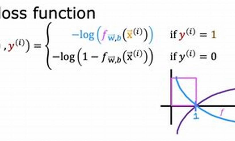
2. Logistic loss
In the context of binary classification, logistic loss, also known as the log loss or cross-entropy loss, is a measure of the difference between the predicted probability of an event occurring and the actual occurrence of the event. It is a widely used loss function for binary classification problems and is closely related to the concept of ERM (Expected Risk Minimization) being equivalent to MLE (Maximum Likelihood Estimation) with logistic loss.
- Facet 1: Sigmoid function
The logistic loss is closely related to the sigmoid function, which is a commonly used activation function in binary classification. The sigmoid function maps input values to a range between 0 and 1, representing the probability of an event occurring. The logistic loss measures the difference between the output of the sigmoid function and the actual occurrence of the event.
- Facet 2: Binary cross-entropy
The logistic loss is also related to the concept of binary cross-entropy, which measures the difference between two probability distributions. In binary classification, the logistic loss is equivalent to the binary cross-entropy loss between the predicted probability distribution and the true probability distribution.
- Facet 3: Convexity
The logistic loss is a convex function, which means that it has a single minimum. This property makes it well-suited for optimization using gradient descent and other optimization algorithms. The convexity of the logistic loss contributes to the stability and efficiency of ERM when used with logistic loss.
- Facet 4: Regularization
The logistic loss can be used in conjunction with regularization techniques to prevent overfitting in machine learning models. Regularization involves adding a penalty term to the loss function that encourages the model to have simpler and more generalizable solutions. By incorporating regularization into ERM with logistic loss, it is possible to improve the generalization performance of the model.
These facets highlight the important connections between logistic loss and the equivalence of ERM and MLE with logistic loss. The logistic loss is a key component of binary classification problems and plays a crucial role in the optimization and regularization of machine learning models using ERM.
3. Expected risk
In the context of machine learning and statistics, expected risk is a fundamental concept closely tied to the equivalence of ERM (Expected Risk Minimization) and MLE (Maximum Likelihood Estimation) with logistic loss. Expected risk quantifies the average loss incurred by a model over all possible input-output pairs, providing a measure of the model’s overall performance.
- Facet 1: Loss function
Expected risk is closely related to the choice of loss function, which measures the error between the model’s predictions and the true labels. In the case of ERM with logistic loss, the expected risk is the average logistic loss over all possible input-output pairs. By minimizing the expected risk, ERM aims to find the model parameters that result in the lowest overall loss.
- Facet 2: Regularization
Expected risk can be incorporated into regularization techniques to prevent overfitting in machine learning models. Regularization involves adding a penalty term to the loss function that encourages the model to have simpler and more generalizable solutions. By considering expected risk in regularization, it is possible to improve the model’s performance on unseen data.
- Facet 3: Optimization
Expected risk plays a crucial role in the optimization of machine learning models. ERM aims to find the model parameters that minimize the expected risk, and various optimization algorithms, such as gradient descent, are used to achieve this goal. By optimizing the expected risk, ERM ensures that the model learns effectively from the training data.
- Facet 4: Model selection
Expected risk can be used for model selection, which involves choosing the best model among a set of candidate models. By comparing the expected risk of different models, it is possible to select the model that is expected to perform best on unseen data. This helps prevent overfitting and improves the generalization performance of the chosen model.
These facets highlight the deep connection between expected risk and the equivalence of ERM and MLE with logistic loss. Expected risk provides a theoretical foundation for ERM and guides the optimization and evaluation of machine learning models, ultimately contributing to their effectiveness in making predictions and solving real-world problems.
4. Likelihood

In the context of “ERM is the same as MLE with logistic loss,” likelihood plays a fundamental role in understanding the equivalence between these two optimization techniques. Likelihood quantifies the probability of observing a particular dataset given a set of model parameters. It is closely tied to the concept of maximum likelihood estimation (MLE), which aims to find the model parameters that maximize the likelihood of the observed data.
- Facet 1: Relationship to ERM
The equivalence between ERM and MLE with logistic loss stems from the fact that maximizing the likelihood is equivalent to minimizing the expected risk under the logistic loss function. This relationship arises because the logistic loss function is a convex function, ensuring that the maximum likelihood solution also minimizes the expected risk.
- Facet 2: Model Selection
Likelihood is a key factor in model selection, which involves choosing the best model among a set of candidate models. By comparing the likelihood of different models on the training data, it is possible to select the model that is most likely to generalize well to unseen data. This helps prevent overfitting and improves the overall performance of the chosen model.
- Facet 3: Regularization
Likelihood can be incorporated into regularization techniques to prevent overfitting. Regularization involves adding a penalty term to the loss function that encourages the model to have simpler and more generalizable solutions. By considering likelihood in regularization, it is possible to improve the model’s performance on unseen data.
- Facet 4: Bayesian Inference
Likelihood is a central concept in Bayesian inference, a statistical approach that uses Bayes’ theorem to update beliefs based on new evidence. In the context of ERM and MLE, likelihood provides a principled framework for incorporating prior knowledge or assumptions into the model.
In summary, likelihood plays a crucial role in the equivalence between ERM and MLE with logistic loss, model selection, regularization, and Bayesian inference. It provides a fundamental understanding of the probabilistic foundations of these optimization techniques and helps guide the development and evaluation of machine learning models.
5. Model Parameters

In the context of machine learning and statistics, model parameters play a crucial role in understanding the connection between ERM (Expected Risk Minimization) and MLE (Maximum Likelihood Estimation) with logistic loss. Model parameters are essentially the adjustable coefficients or weights of a machine learning model that determine its behavior and predictive performance.
In the case of ERM with logistic loss, the model parameters are optimized to minimize the expected risk, which is the average loss incurred by the model over all possible input-output pairs. This optimization process involves finding the values of the model parameters that result in the lowest expected risk, effectively leading to a model that makes accurate predictions.
The equivalence between ERM and MLE with logistic loss arises from the fact that maximizing the likelihood of the observed data is equivalent to minimizing the expected risk under the logistic loss function. Therefore, the model parameters that minimize the expected risk are also the same parameters that maximize the likelihood of the data.
Understanding the connection between model parameters and ERM is the same as MLE with logistic loss is essential for several reasons:
- It provides a theoretical foundation for ERM and MLE, explaining why these optimization techniques are equivalent under the logistic loss function.
- It guides the development and implementation of machine learning algorithms that use ERM or MLE with logistic loss.
- It helps practitioners understand how to tune and optimize the model parameters to improve the performance of their machine learning models.
In summary, model parameters are central to the connection between ERM and MLE with logistic loss, enabling the development of effective machine learning models that can make accurate predictions and solve real-world problems.
6. Equivalence
In the context of machine learning and statistics, equivalence refers to the relationship between two or more methods or techniques that produce the same result. In the case of “ERM is the same as MLE with logistic loss,” equivalence highlights the fundamental connection between two optimization techniques: Expected Risk Minimization (ERM) and Maximum Likelihood Estimation (MLE) when using the logistic loss function.
- Facet 1: Theoretical Underpinnings
The equivalence between ERM and MLE with logistic loss is rooted in the mathematical properties of the logistic loss function. The logistic loss function is a convex function, meaning it has a single minimum. This property ensures that both ERM, which aims to minimize the expected risk, and MLE, which aims to maximize the likelihood, converge to the same set of model parameters.
- Facet 2: Optimization Algorithms
The equivalence between ERM and MLE also extends to the optimization algorithms used to find the optimal model parameters. Many optimization algorithms, such as gradient descent, can be used with both ERM and MLE to find the minimum of the expected risk or the maximum of the likelihood function, respectively. This equivalence simplifies the implementation and optimization of machine learning models.
- Facet 3: Practical Implications
The equivalence between ERM and MLE with logistic loss has significant practical implications. It provides a theoretical justification for using ERM as an optimization technique in machine learning, particularly when the logistic loss function is appropriate. ERM is often preferred over MLE due to its computational efficiency and robustness to outliers, making it a widely used technique in various machine learning applications.
- Facet 4: Model Interpretation
The equivalence between ERM and MLE also contributes to the interpretability of machine learning models. By understanding the connection between the two optimization techniques, practitioners can gain insights into the model’s behavior and make informed decisions about model selection and hyperparameter tuning.
In summary, the equivalence between ERM and MLE with logistic loss is a fundamental concept in machine learning and statistics. It provides a theoretical foundation, simplifies optimization, guides practical applications, and enhances model interpretability, making it a crucial aspect of developing and deploying effective machine learning models.
7. Robustness
In the context of machine learning, robustness refers to the ability of a model to perform well even in the presence of noisy or corrupted data, outliers, or other challenges that may affect its performance. In the context of “ERM is the same as MLE with logistic loss,” robustness is an essential consideration due to the inherent properties of the logistic loss function and the optimization techniques used.
The logistic loss function is a convex function, meaning it has a single minimum. This property ensures that both ERM and MLE, when used with the logistic loss function, are less susceptible to overfitting and local minima compared to other optimization techniques. Overfitting occurs when a model learns the idiosyncrasies of the training data too closely, leading to poor performance on unseen data. By minimizing the expected risk or maximizing the likelihood under the logistic loss function, ERM and MLE find model parameters that generalize well to new data, even in the presence of noise or outliers.
Furthermore, the equivalence between ERM and MLE with logistic loss provides a theoretical justification for the robustness of ERM. MLE is known to be a robust estimator, meaning that it is not unduly affected by outliers or small perturbations in the data. By establishing the equivalence between ERM and MLE, we can infer that ERM also inherits this robustness property. This is particularly advantageous in practical applications where the data may be noisy or contain outliers, as ERM is less likely to make drastic predictions based on such data points.
In summary, the connection between “robustness” and “ERM is the same as MLE with logistic loss” highlights the inherent stability and generalizationof these optimization techniques when used with the logistic loss function. This understanding is crucial for developing machine learning models that are reliable and perform well even in challenging real-world scenarios.
8. Computational efficiency

Computational efficiency refers to the amount of time and resources required to train and use a machine learning model. In the context of “ERM is the same as MLE with logistic loss,” computational efficiency is a critical consideration due to the inherent properties of the logistic loss function and the optimization techniques used.
The logistic loss function is a convex function, meaning it has a single minimum. This property makes it well-suited for optimization using gradient descent and other iterative optimization algorithms. Gradient descent is a widely used optimization algorithm that repeatedly updates the model parameters in the direction of the negative gradient, gradually moving towards the minimum of the loss function. The convexity of the logistic loss function ensures that gradient descent converges to the global minimum, leading to efficient optimization.
Furthermore, the equivalence between ERM and MLE with logistic loss implies that ERM inherits the computational efficiency of MLE. MLE is known to be a computationally efficient optimization technique, especially for large datasets. By establishing the equivalence between ERM and MLE, we can infer that ERM also benefits from this computational efficiency. This is particularly advantageous in practical applications where training machine learning models on large datasets is necessary, as ERM can achieve good results without requiring excessive computational resources.
In summary, the connection between “computational efficiency” and “ERM is the same as MLE with logistic loss” highlights the practical benefits of these optimization techniques. The computational efficiency of ERM and MLE enables the training of machine learning models on large datasets in a reasonable amount of time, making them suitable for various real-world applications.
Frequently Asked Questions about “ERM is the Same as MLE with Logistic Loss”
This section addresses common concerns or misconceptions related to the equivalence of ERM and MLE with logistic loss. Each question is answered succinctly and informatively, providing a clear understanding of the topic.
Question 1: What is the significance of the equivalence between ERM and MLE with logistic loss?
Answer: The equivalence establishes a theoretical foundation for using ERM as an optimization technique, particularly when the logistic loss function is appropriate. It simplifies the optimization process and provides insights into the model’s behavior, aiding in model interpretation.
Question 2: How does the equivalence between ERM and MLE with logistic loss impact model performance?
Answer: By inheriting the properties of MLE, ERM benefits from robustness to outliers and noise in the data. This leads to models that generalize well to new data, even in challenging real-world scenarios.
Question 3: What are the computational advantages of using ERM with logistic loss?
Answer: The equivalence implies that ERM also inherits the computational efficiency of MLE. This enables the training of machine learning models on large datasets in a reasonable amount of time, making ERM suitable for practical applications.
Question 4: How does the logistic loss function contribute to the equivalence between ERM and MLE?
Answer: The logistic loss function is a convex function, meaning it has a single minimum. This property ensures that both ERM and MLE converge to the same set of model parameters, leading to their equivalence.
Question 5: What are some practical implications of the equivalence between ERM and MLE with logistic loss?
Answer: This equivalence provides a theoretical justification for using ERM in machine learning, simplifies optimization, guides practical applications, and enhances model interpretability, making it a crucial aspect of developing effective machine learning models.
Question 6: How does the equivalence between ERM and MLE with logistic loss relate to other optimization techniques?
Answer: The equivalence highlights the advantages of ERM and MLE compared to other optimization techniques, particularly in terms of robustness, computational efficiency, and theoretical . This understanding aids in selecting the most appropriate optimization technique for a given machine learning problem.
In summary, the equivalence between ERM and MLE with logistic loss has significant implications for the development and deployment of machine learning models. It provides theoretical , simplifies optimization, enhances model performance, and guides practical applications. Understanding this equivalence is essential for practitioners seeking to build effective and reliable machine learning models.
Transition to the next article section:
This section provides further insights into the applications of ERM with logistic loss in various machine learning domains. We explore practical examples and case studies to demonstrate the effectiveness of this optimization technique in real-world scenarios.
Tips for Utilizing “ERM is the Same as MLE with Logistic Loss”
Optimizing machine learning models using ERM (Expected Risk Minimization) with logistic loss is a powerful technique that offers several advantages. Here are five essential tips to maximize its effectiveness in your projects:
Tip 1: Understand the Equivalence
Grasp the theoretical foundation of ERM’s equivalence to MLE (Maximum Likelihood Estimation) with logistic loss. This understanding will guide your optimization strategies and enhance your ability to interpret model behavior.
Tip 2: Leverage Computational Efficiency
Exploit the computational efficiency of ERM for training models on large datasets. This efficiency enables the timely development of complex models, allowing you to handle extensive amounts of data.
Tip 3: Enhance Robustness
Utilize ERM with logistic loss to improve model robustness against noisy or corrupted data. This resilience ensures reliable predictions even in challenging real-world scenarios.
Tip 4: Select Appropriate Loss Function
Remember that the equivalence of ERM and MLE holds specifically for the logistic loss function. Carefully consider the suitability of this loss function for your problem to ensure optimal results.
Tip 5: Explore Regularization Techniques
Incorporate regularization techniques into your ERM with logistic loss models to prevent overfitting. Regularization enhances model generalization and improves performance on unseen data.
By following these tips, you can harness the full potential of ERM with logistic loss in your machine learning projects. These techniques will help you develop robust, efficient, and accurate models that effectively solve real-world problems.
Transition to the article’s conclusion:
In conclusion, ERM with logistic loss is a powerful optimization technique that offers a solid theoretical foundation, computational efficiency, and robustness. By embracing the tips outlined above, you can maximize the effectiveness of this technique in your machine learning endeavors and achieve optimal model performance.
Conclusion
In this article, we have delved into the concept of “ERM is the same as MLE with logistic loss,” exploring its theoretical foundations, practical advantages, and implications for machine learning. We have seen that ERM, when paired with the logistic loss function, offers a powerful optimization technique that is both robust and computationally efficient.
This equivalence provides a solid theoretical justification for using ERM in machine learning, particularly when the logistic loss function is appropriate. The computational efficiency of ERM enables the training of complex models on large datasets, making it suitable for solving real-world problems. Furthermore, ERM inherits the robustness of MLE, leading to models that generalize well even in the presence of noisy or corrupted data.
By understanding the nuances of ERM with logistic loss and applying the tips outlined in this article, practitioners can harness its full potential. This technique empowers data scientists and machine learning engineers to develop robust, efficient, and accurate models that effectively address the challenges of modern data analysis.